
はじめに
前回は、両端固定された1次元棒を題材に、等方線形硬化を入れた熱弾塑性解析を整理しました。線形硬化では、塑性変形が蓄積するほど降伏応力が大きくなり、材料がさらに塑性変形しにくくなる様子を表しました。
今回は、硬化とは別の重要な効果として、降伏応力の温度依存性を扱います。金属材料では、温度が高くなると降伏応力が低下することがあります。つまり、同じ応力でも、低温では弾性範囲に収まっていた状態が、高温では降伏条件に達することがあります。この記事では、まず温度依存の降伏応力を理論式として入れます。
その後で、両端固定棒の加熱・冷却を数値実験し、温度依存性を入れると応力履歴や塑性ひずみがどう変わるかを確認します。狙いは、材料点レベルで
- 降伏応力が温度で下がるとは何を意味するのか
- 降伏条件が温度を含むとどう変わるのか
- 温度依存性が降伏開始温度や応力履歴にどう効くのか
- まずは硬化と温度依存性を分けて理解すること
を見通せるようにすることです。

モデル化する問題
対象はこれまでと同じく、両端固定された長さ \(L_0\) の1次元棒です。両端が固定されているので、棒全体としての軸方向ひずみは
\varepsilon = 0 \tag{1}
\end{align}
です。この式は、棒が全体として伸び縮みできないことを表しています。温度が上がると材料は自由膨張しようとしますが、その変形が拘束されるため、棒の中には圧縮側の熱応力が生じます。
今回の仮定は次の通りです。
- 1次元棒として扱います。
- 温度は棒全体で一様です。
- 全ひずみは両端固定により常にゼロです。
- ヤング率 \(E\) と線膨張係数 \(\alpha\) は一定とします。
- 降伏応力だけを温度依存にします。
- まずは硬化を入れず、完全弾塑性モデルとして扱います。
ここで硬化を入れないのは、温度依存性の影響だけを切り出して見るためです。線形硬化と温度依存性を同時に入れることもできますが、最初から両方を入れると、どちらの効果で応答が変わったのかが見えにくくなります。
ひずみの分解
熱弾塑性解析では、全ひずみを弾性ひずみ、塑性ひずみ、熱ひずみに分けます。
\varepsilon =\varepsilon_e+\varepsilon_p+\varepsilon_{\mathrm{th}} \tag{2}
\end{align}
この式は、観測される全ひずみを、応力を生む弾性ひずみ、戻らない塑性ひずみ、温度変化だけで生じる熱ひずみに分けて考えるという意味です。
熱ひずみは
\varepsilon_{\mathrm{th}}
=\alpha \Delta T \tag{3}
\end{align}
です。これは、拘束がなければ温度上昇に比例して棒が自由に伸びることを表しています。
一方、今回の棒は両端固定なので、式(1)と式(2)より
\varepsilon_e =-\varepsilon_p-\varepsilon_{\mathrm{th}} \tag{4}
\end{align}
となります。
温度が上がって熱ひずみが正になると、それを打ち消すように弾性ひずみは負になります。応力はフックの法則
\sigma=E\varepsilon_e \tag{5}
\end{align}
で決まるため、加熱中には圧縮側の応力が生じます。
温度依存の降伏応力
完全塑性モデルでは、降伏応力を一定値 \(\sigma_Y\) として扱いました。しかし実際の材料では、温度が高くなるほど降伏応力が低下する場合があります。この理由を、金属材料をイメージして考えます。
金属の塑性変形は、原子面全体が一斉にずれるというより、主に転位が材料内部を移動することで進みます。転位が動くときには、結晶格子そのものによる抵抗、固溶原子、析出物、粒界、ほかの転位などが障害になります。低温では、これらの障害を越えるためのエネルギーを主に外力による応力で与える必要があるため、大きな応力をかけないと塑性変形が始まりません。
一方、温度が上がると原子の熱振動が大きくなり、転位が障害を越える過程を熱エネルギーが助けます。このように、外力だけでなく熱によって変形過程が進みやすくなる性質は、熱活性化過程として理解できます。その結果、同じ塑性変形を開始するために必要な外部応力は小さくなり、見かけの降伏応力は低下します。
さらに高温では、拡散、回復、転位の上昇運動なども起こりやすくなるため、材料の変形抵抗はより下がりやすくなります。ただし、実際の降伏応力の温度依存性は、材料、温度範囲、ひずみ速度、熱処理や組織状態によって変わります。
そのため、本記事では物理機構を厳密に表す構成式を作るのではなく、温度上昇によって降伏応力が下がる効果を学ぶための最も単純な近似として、温度変化 \(\Delta T\) に対して降伏応力が直線的に低下すると考えます。
\sigma_Y(\Delta T)=\sigma_{Y0}\left(1-\beta \Delta T\right) \tag{6}
\end{align}
ここで、\(\sigma_{Y0}\) は基準温度での降伏応力、\(\beta\) は降伏応力の温度低下率です。式(6)は、温度が上がるほど材料が降伏しやすくなることを表しています。
ただし、この式は簡易モデルなので、高温までそのまま外挿すると降伏応力がゼロや負になる可能性があります。実装では必要に応じて下限値を設けます。この効果を応力-ひずみ線図で見ると、図1のようになります。
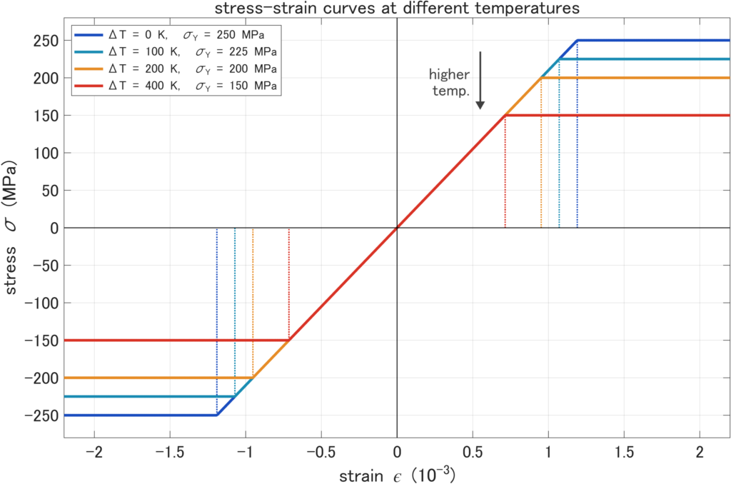
ヤング率 \(E\) はここでは温度によらず一定としたので、原点近くの弾性勾配はどの温度でも同じです。一方、温度が上がるほど \(\sigma_Y(\Delta T)\) が小さくなるため、弾性直線から塑性域へ移る降伏点は原点側へ近づきます。
つまり、温度上昇は「同じひずみまで弾性的に耐えられる範囲を狭くする」効果としてSSカーブ上に現れます。1次元の降伏条件は、温度依存の降伏応力を使って
f(\sigma,\Delta T)=|\sigma|-\sigma_Y(\Delta T)\le 0 \tag{7}
\end{align}
と書けます。絶対値が入っているのは、引張側でも圧縮側でも、応力の大きさが現在温度での降伏応力に達したら降伏すると考えるためです。
加熱された固定棒では圧縮側に応力が進むので、最初に問題になるのは
\sigma=-\sigma_Y(\Delta T) \tag{8}
\end{align}
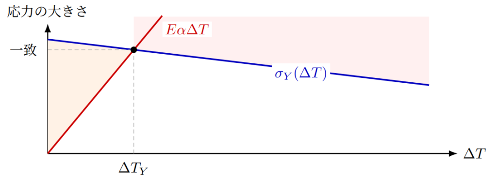
に到達するかどうかです。つまり、温度依存性を入れると、温度上昇によって圧縮応力が増えるだけでなく、同時に圧縮側の降伏限界も材料側から近づいてきます。
降伏開始温度
塑性ひずみがまだ生じていない初期状態では、\(\varepsilon_p=0\) です。両端固定なので、式(4)より
\varepsilon_e=-\alpha \Delta T \tag{9}
\end{align}
となります。したがって、弾性範囲での圧縮応力の大きさは
|\sigma|=E\alpha\Delta T \tag{10}
\end{align}
です。温度依存の降伏応力を入れると、降伏開始は
E\alpha\Delta T_Y=\sigma_{Y0}\left(1-\beta \Delta T_Y\right) \tag{11}
\end{align}
で決まります。左辺は温度上昇によって生じる圧縮熱応力の大きさ、右辺はその温度での降伏応力です。温度依存性がない場合は右辺が一定ですが、温度依存性がある場合は右辺も温度とともに小さくなります。そのため、降伏開始温度は低くなります。
式(11)を \(\Delta T_Y\) について解くと、
\Delta T_Y=\frac{\sigma_{Y0}}{E\alpha+\sigma_{Y0}\beta} \tag{12}
\end{align}
となります。分母に \(\sigma_{Y0}\beta\) が加わるため、\(\beta=0\) の場合よりも降伏開始温度が小さくなることが分かります。
応力更新アルゴリズム
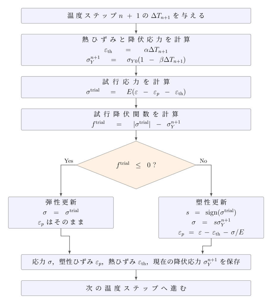
数値解析では、温度履歴を小さなステップに分け、各ステップで応力と塑性ひずみを更新します。まず、現在の塑性ひずみを固定したまま、弾性で進んだと仮定した試行応力を計算します
\sigma^{\mathrm{trial}} =E\left(\varepsilon-\varepsilon_p-\varepsilon_{\mathrm{th}}\right) \tag{13}
\end{align}
これは、今回の温度ステップを塑性変形なしで進めたらどの応力になるか、という予測です。次に、その温度での降伏応力
\sigma_Y^{n+1}=\sigma_Y(\Delta T_{n+1}) \tag{14}
\end{align}
を計算し、試行降伏関数
f^{\mathrm{trial}}=|\sigma^{\mathrm{trial}}|-\sigma_Y^{n+1} \tag{15}
\end{align}
を評価します。もし \(f^{\mathrm{trial}}\le0\) なら、試行応力は現在温度での降伏範囲内にあります。そのため、応力は
\sigma=\sigma^{\mathrm{trial}} \tag{16}
\end{align}
であり、塑性ひずみは更新しません。
一方、\(f^{\mathrm{trial}}>0\) なら、試行応力は降伏範囲の外に出ています。完全塑性なので、応力は現在温度での降伏応力に戻します。1次元では、試行応力の符号を
s=\mathrm{sign}\left(\sigma^{\mathrm{trial}}\right) \tag{17}
\end{align}
とすれば、更新後の応力は
\sigma=s\sigma_Y^{n+1} \tag{18}
\end{align}
です。圧縮側で降伏していれば \(s=-1\) なので、\(\sigma=-\sigma_Y^{n+1}\) になります。塑性ひずみは、更新後の応力とひずみ分解式が整合するように
\varepsilon_p^{\mathrm{new}}=\varepsilon-\varepsilon_{\mathrm{th}}-\frac{\sigma}{E} \tag{19}
\end{align}
と更新します。この式は、全ひずみと熱ひずみが決まっている状況で、応力から弾性ひずみを逆算し、残りを塑性ひずみとして保存するという意味です。
解析条件
ここまでで、温度依存の降伏応力を入れたときの定式化と応力更新手順を整理しました。ここからは、その定式化を使った数値例に移ります。この節では、まだ計算結果の解釈には入らず、温度履歴、材料定数、数値計算で用いる条件を整理します。
温度履歴と材料定数
数値例では、温度を \(0\) K から \(400\) K まで上げ、その後 \(0\) K まで戻します。材料定数と解析条件は次の通りです。
\begin{array}{c}
\text{表: 数値例で用いる材料定数と解析条件。} \\
\begin{array}{ccl}
\hline
\text{記号} & \text{値} & \text{意味} \\
\hline
E & 210000\,\mathrm{MPa} & \text{ヤング率} \\
\alpha & 12\times10^{-6}\,\mathrm{K}^{-1} & \text{線膨張係数} \\
\sigma_{Y0} & 250\,\mathrm{MPa} & \text{基準温度での降伏応力} \\
\beta & 1.0\times10^{-3}\,\mathrm{K}^{-1} & \text{降伏応力の温度低下率} \\
\Delta T_{\max} & 400\,\mathrm{K} & \text{最大温度上昇} \\
\hline
\end{array}
\end{array}
\end{align}
降伏開始温度の事前見積もり
この条件では、温度依存性を入れない場合の降伏開始温度は
\Delta T_Y=\frac{\sigma_{Y0}}{E\alpha}\simeq 99.2\ \mathrm{K} \tag{20}
\end{align}
です。一方、温度依存性を入れると、式(12)より
\Delta T_Y =\frac{250}{210000\times12\times10^{-6}+250\times10^{-3}}\simeq 90.3\ \mathrm{K} \tag{21}
\end{align}
となります。降伏応力が温度とともに下がるため、より低い温度で降伏が始まります。
数値計算で用いる更新条件
数値計算では、同じ温度履歴に対して、降伏応力一定の場合と温度依存性ありの場合を比較します。各温度ステップで、まず熱ひずみと現在温度での降伏応力を計算し、試行応力を作ってから降伏判定を行います。温度依存性ありのケースでは、降伏応力を
\sigma_Y(\Delta T)=\max\left[50,\,\sigma_{Y0}\left(1-\beta\Delta T\right)\right]\tag{22}
\end{align}
として計算しています。今回の温度範囲では下限値 \(50\) MPa には達しませんが、簡易式を高温側へ外挿したときに降伏応力が負にならないようにするための処理です。
計算結果
ここから先は、前節の条件で得られる計算結果です。理論式で予想した降伏開始温度が、離散化された温度ステップの計算でどのように現れるか、また応力履歴とひずみ履歴がどのように変わるかを確認します。
代表値の確認
まず、降伏開始温度、最大温度での応力、冷却後の残留応力を代表値として整理します。理論式では、温度依存性ありの降伏開始温度は約 \(90.3\) K でした。数値計算では、温度履歴を \(2\) K刻みで与えているため、最初に降伏条件を超える温度ステップは \(92.00\) K になります。実際の降伏開始は \(90.3\) K付近ですが、離散化された温度ステップの中で最初に降伏条件を超える点が \(92\) Kになります。
\begin{array}{c}
\text{表: 温度依存性なしと温度依存性ありの比較。} \\
\begin{array}{ccl}
\hline
\text{項目} & \text{温度依存性なし} & \text{温度依存性あり} \\
\hline
\text{降伏開始温度} & \text{約}99.2\,\mathrm{K} & \text{約}90.3\,\mathrm{K} \\
\text{最大温度での降伏応力} & 250\,\mathrm{MPa} & 150\,\mathrm{MPa} \\
\text{最大温度での応力} & -250\,\mathrm{MPa} & -150\,\mathrm{MPa} \\
\text{冷却後の残留応力} & 250\,\mathrm{MPa} & \text{約}250\,\mathrm{MPa} \\
\hline
\end{array}
\end{array}
\end{align}
降伏開始温度と最大温度での応力
図4は最終的な履歴を一枚にまとめたものです。現在の温度ステップを点で示しながら、応力、降伏応力、塑性ひずみがどのように変化するかを確認できます。
まず分かりやすい違いは、降伏開始温度です。温度依存性なしでは、圧縮熱応力の大きさが \(250\) MPa に達するまで降伏しません。温度依存性ありでは、温度上昇とともに降伏応力そのものが下がるため、約 \(90.3\) K で降伏が始まります。
次に、最大温度での応力です。温度依存性なしの場合、完全塑性なので加熱中の圧縮応力は \(-250\) MPa に張り付きます。一方、温度依存性ありの場合、\(400\) K での降伏応力は
\sigma_Y(400)=250\left( 1 – 1.0\times10^{-3}\times400\right) =150\ \mathrm{MPa} \tag{23}
\end{align}
です。そのため、最大温度付近では圧縮応力も \(-150\) MPa 程度まで小さくなります。ここが、温度依存性を入れたときの最も見えやすい効果です。降伏応力が小さくなることによって、早い段階で降伏するようになるので、その分塑性ひずみの開始点が早くなり最大塑性ひずみが大きくなります。
また、今回の1次元・両端固定・完全弾塑性モデルでは、温度依存性に問わず最終的な残留応力はほぼ変わりません。理由は、冷却して最後に \(\Delta T=0\) に戻ると、降伏応力も基準温度の値
\sigma_Y(0)=\sigma_{Y0}=250\,\mathrm{MPa} \tag{24}
\end{align}
に戻るからです。加熱中は温度依存性によって高温側の降伏応力が下がるので、最大温度付近の圧縮応力は小さくなります。しかし冷却中に温度が下がると、降伏応力はまた大きくなります。両端固定なので全ひずみはゼロのままですから、冷却過程では弾性ひずみが引張側へ戻っていき、最終的には引張側の降伏応力付近に張り付きます。つまり今回のモデルでは、\( \sigma_{\mathrm{final}} \simeq +\sigma_{Y0} \)になりやすいです。
ただし、「残留応力が必ず変わらない」という意味ではありません。温度依存性を入れると、途中の応力履歴、塑性ひずみの進み方、最大温度での応力は変わります。さらに硬化、温度依存するヤング率、温度依存する熱膨張係数、応力緩和、クリープ、非一様温度場などを入れると、最終残留応力も変わり得ます。今回変わりにくいのは、かなり単純化した完全弾塑性モデルだからです。
同じ結果をSSカーブ上で見ると、温度によって材料側の降伏応力が変わることと、熱負荷による応力経路が別のものだと分かりやすくなります。図5では温度ごとのSSカーブを背景に置き、その上に固定棒の加熱・冷却で得られた応力経路を重ねています。
材料試験のSSカーブをそのままたどっているのではなく、熱拘束によって生じた応力状態が、温度依存の降伏面に制限されながら動いている、と見るのがポイントです。
冷却後の残留応力とひずみ成分
冷却後の残留応力については、今回の単純な条件ではどちらも引張側の降伏応力に近い値になります。ただし、そこに至るまでの履歴は異なります。温度依存性ありの場合、加熱中は高温で材料が弱くなるため、低い圧縮応力で塑性変形が進みます。その後、冷却によって降伏応力が回復し、最終的には基準温度の降伏応力に近い引張残留応力が残ります。
ひずみ成分だけを取り出すと、図6のようになります。
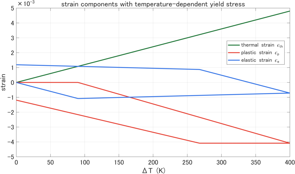
熱ひずみは温度だけで決まるため、加熱時と冷却時で同じ直線上を通ります。一方、塑性ひずみと弾性ひずみは履歴量を含むため、同じ温度でも加熱時と冷却時で異なる値になります。これは、温度依存の降伏応力を入れても、熱弾塑性解析では履歴を保存する必要があることを示しています。
図7では、熱ひずみ、塑性ひずみ、弾性ひずみを温度に対して分けて表示しています。
熱ひずみは温度だけで決まるので、加熱時も冷却時も同じ線上を通ります。一方で、塑性ひずみと弾性ひずみは履歴を持つため、同じ温度に戻ってきても同じ値にはなりません。この違いを見ると、熱弾塑性解析で状態変数を更新しながら進める必要があることが分かります。
このモデルから分かること
温度依存の降伏応力を入れると、熱弾塑性解析の中で温度が二つの役割を持つことが分かります。
一つ目は、熱ひずみを通じて応力を発生させる役割です。温度が上がるほど自由膨張したい量が増え、固定棒では圧縮応力が大きくなります。
二つ目は、材料の降伏しやすさを変える役割です。温度が上がるほど降伏応力が低下するなら、材料はより小さい応力で塑性変形を始めます。つまり、加熱は「応力を作る原因」であると同時に、「材料を降伏しやすくする原因」でもあります。
この二つが同時に働くため、温度依存性を入れた熱弾塑性解析では、一定降伏応力モデルよりも早く降伏が始まり、高温域での応力レベルが小さくなります。この効果は、溶接、熱処理、積層造形のように温度変化が大きい問題で特に重要になります。
線形硬化との組み合わせ
今回のモデルでは、温度依存性の効果だけを見るために硬化を入れませんでした。しかし次の段階では、前回扱った等方線形硬化と今回の温度依存降伏応力を組み合わせも考えられます。その場合、降伏応力は例えば
\sigma_Y(\Delta T,\kappa)=\sigma_{Y0}\left(1 – \beta\Delta T\right)+H\kappa \tag{24}
\end{align}
のように表せます。この式では、温度上昇は降伏応力を下げ、塑性変形の蓄積は降伏応力を上げます。二つの効果が逆向きに働くため、履歴の解釈は少し複雑になります。だからこそ、今回のように温度依存性だけを先に切り出して理解しておくと、次の拡張が追いやすくなります。
MATLABコード
今回使用したコードを以下に記載します。
% temperature_dependent_yield_demo.m
% 温度依存の降伏応力を持つ1次元熱弾塑性モデルの最小計算例です。
% 両端固定棒を 0 -> 400 K -> 0 K と加熱・冷却し、
% 降伏応力一定の場合と、降伏応力が温度で低下する場合を比較します。

clear; close all; clc;

% ---- 材料定数と解析条件 ----
E = 210000;              % MPa, ヤング率
alpha = 12e-6;           % 1/K, 線膨張係数
sigmaY0 = 250;           % MPa, 基準温度での降伏応力
beta = 1.0e-3;           % 1/K, 降伏応力の温度低下率
Tmax = 400;              % K, 最大温度上昇
nHalf = 200;             % 加熱側の分割数
saveMp4 = true;          % ブログ用MP4を保存するか
saveResponseMp4 = true;
saveStressStrainMp4 = true;
saveStrainTemperatureMp4 = true;
videoFrameRate = 15;     % fps
animationStride = 4;     % 何ステップごとに描画するか

responseMp4FileName = "temperature_dependent_yield_response_animation.mp4";
stressStrainMp4FileName = "temperature_dependent_yield_stress_strain_path.mp4";
strainTemperatureMp4FileName = "temperature_dependent_yield_strain_temperature_path.mp4";

% 温度履歴: 0 -> Tmax -> 0
T_up = linspace(0, Tmax, nHalf + 1);
T_down = linspace(Tmax, 0, nHalf + 1);
dT = [T_up, T_down(2:end)];
step = 0:numel(dT)-1;

% 2ケースを計算します。
caseConst = run_case(dT, E, alpha, sigmaY0, beta, false);
caseTemp = run_case(dT, E, alpha, sigmaY0, beta, true);

% ---- 代表値を表示 ----
fprintf('=== Constant yield stress ===\n');
fprintf('Initial yield temperature = %.2f K\n', caseConst.initialYieldTemperature);
fprintf('Stress at Tmax = %.3f MPa\n', caseConst.stressAtTmax);
fprintf('Final stress = %.3f MPa\n', caseConst.sigma(end));
fprintf('Final plastic strain = %.6e\n', caseConst.epsP(end));
fprintf('Yield stress at Tmax = %.3f MPa\n', caseConst.sigmaYAtTmax);

fprintf('\n=== Temperature-dependent yield stress ===\n');
fprintf('Initial yield temperature = %.2f K\n', caseTemp.initialYieldTemperature);
fprintf('Stress at Tmax = %.3f MPa\n', caseTemp.stressAtTmax);
fprintf('Final stress = %.3f MPa\n', caseTemp.sigma(end));
fprintf('Final plastic strain = %.6e\n', caseTemp.epsP(end));
fprintf('Yield stress at Tmax = %.3f MPa\n', caseTemp.sigmaYAtTmax);

% ---- 図: 温度によるSSカーブの変化 ----
% ここでは単調な材料試験を想定した模式的な応力--ひずみ曲線を描きます。
% 温度が上がるほど降伏応力が低下するため、弾性直線から塑性域へ移る点が内側に寄ります。
temperatureLevels = [0, 100, 200, 400];     % K
epsAxis = linspace(-0.0022, 0.0022, 600);   % 全ひずみ
colors = [0.10 0.30 0.75;
          0.10 0.55 0.70;
          0.90 0.55 0.15;
          0.85 0.20 0.15];

figSS = figure('Color', 'w', 'Position', [140 140 1200 720]);
hold on;
for k = 1:numel(temperatureLevels)
    Tlevel = temperatureLevels(k);
    sigmaYLevel = max(50, sigmaY0 * (1 - beta * Tlevel));
    sigmaCurve = min(max(E * epsAxis, -sigmaYLevel), sigmaYLevel);
    plot(epsAxis * 1000, sigmaCurve, 'LineWidth', 2.8, ...
        'Color', colors(k, :), ...
        'DisplayName', sprintf('\\DeltaT = %d K,  \\sigma_Y = %.0f MPa', Tlevel, sigmaYLevel));

    epsYLevel = sigmaYLevel / E;
    plot([epsYLevel epsYLevel] * 1000, [0 sigmaYLevel], ':', ...
        'LineWidth', 1.4, 'Color', colors(k, :), 'HandleVisibility', 'off');
    plot([-epsYLevel -epsYLevel] * 1000, [-sigmaYLevel 0], ':', ...
        'LineWidth', 1.4, 'Color', colors(k, :), 'HandleVisibility', 'off');
end

plot([0 0], [-280 280], 'k-', 'LineWidth', 0.8, 'HandleVisibility', 'off');
plot(xlim, [0 0], 'k-', 'LineWidth', 0.8, 'HandleVisibility', 'off');
grid on; box on;
xlabel('strain \epsilon (10^{-3})');
ylabel('stress \sigma (MPa)');
title('stress-strain curves at different temperatures');
xlim([-2.2 2.2]);
ylim([-280 280]);
legend('Location', 'northwest', 'FontSize', 13);
set(gca, 'FontSize', 18);
text(0.48, 195, {'higher', 'temp.'}, 'FontSize', 17, ...
    'HorizontalAlignment', 'right', 'Color', [0.25 0.25 0.25]);
plot([0.55 0.55], [235 165], '-', 'Color', [0.25 0.25 0.25], ...
    'LineWidth', 1.8, 'HandleVisibility', 'off');
plot(0.55, 165, 'v', 'MarkerSize', 8, 'MarkerFaceColor', [0.25 0.25 0.25], ...
    'MarkerEdgeColor', [0.25 0.25 0.25], 'HandleVisibility', 'off');
exportgraphics(figSS, 'temperature_dependent_yield_ss_curves.png', 'Resolution', 220);

% ---- 図1: 計算結果の概要 ----
fig = figure('Color', 'w', 'Position', [100 100 1300 980]);
tiledlayout(2, 2, 'Padding', 'loose', 'TileSpacing', 'loose');

nexttile;
plot(step, dT, 'k-', 'LineWidth', 2.2);
grid on; box on;
xlabel('step');
ylabel('\DeltaT (K)');
title('temperature history');
set(gca, 'FontSize', 16);

nexttile;
plot(dT, caseConst.sigma, 'Color', [0.2 0.45 0.9], 'LineWidth', 2.2); hold on;
plot(dT, caseTemp.sigma, 'Color', [0.9 0.25 0.2], 'LineWidth', 2.2);
plot(dT, -caseTemp.sigmaY, '--', 'Color', [0.55 0.1 0.1], 'LineWidth', 1.8);
plot(dT, caseTemp.sigmaY, '--', 'Color', [0.55 0.1 0.1], 'LineWidth', 1.8);
grid on; box on;
xlabel('\DeltaT (K)');
ylabel('\sigma (MPa)');
title('stress - temperature');
ylim([-310 310]);
legend({'constant \sigma_Y', 'temperature-dependent \sigma_Y', '\pm\sigma_Y(\DeltaT)'}, ...
    'Location', 'southoutside', 'Orientation', 'horizontal', 'FontSize', 11);
set(gca, 'FontSize', 16);

nexttile;
plot(dT, caseConst.sigmaY, 'Color', [0.2 0.45 0.9], 'LineWidth', 2.2); hold on;
plot(dT, caseTemp.sigmaY, 'Color', [0.9 0.25 0.2], 'LineWidth', 2.2);
grid on; box on;
xlabel('\DeltaT (K)');
ylabel('\sigma_Y (MPa)');
title('yield stress');
legend({'constant', 'temperature-dependent'}, ...
    'Location', 'southwest', 'FontSize', 12);
set(gca, 'FontSize', 16);

nexttile;
plot(dT, caseConst.epsP, 'Color', [0.2 0.45 0.9], 'LineWidth', 2.2); hold on;
plot(dT, caseTemp.epsP, 'Color', [0.9 0.25 0.2], 'LineWidth', 2.2);
grid on; box on;
xlabel('\DeltaT (K)');
ylabel('\epsilon_p');
title('plastic strain - temperature');
legend({'constant \sigma_Y', 'temperature-dependent \sigma_Y'}, ...
    'Location', 'southoutside', 'Orientation', 'horizontal', 'FontSize', 12);
set(gca, 'FontSize', 16);

exportgraphics(fig, 'temperature_dependent_yield_summary.png', 'Resolution', 220);

% ---- 図2: ひずみ成分の比較 ----
fig2 = figure('Color', 'w', 'Position', [120 120 1200 620]);
plot(dT, caseTemp.epsTh, 'Color', [0.1 0.45 0.2], 'LineWidth', 2.3); hold on;
plot(dT, caseTemp.epsP, 'Color', [0.9 0.25 0.2], 'LineWidth', 2.3);
plot(dT, caseTemp.epsE, 'Color', [0.2 0.45 0.9], 'LineWidth', 2.3);
grid on; box on;
xlabel('\DeltaT (K)');
ylabel('strain');
title('strain components with temperature-dependent yield stress');
legend({'thermal strain \epsilon_{th}', 'plastic strain \epsilon_p', 'elastic strain \epsilon_e'}, ...
    'Location', 'best', 'FontSize', 14);
set(gca, 'FontSize', 17);
exportgraphics(fig2, 'temperature_dependent_yield_strain_components.png', 'Resolution', 220);

% ---- ブログ用アニメーション1: 計算結果の概要 ----
if saveMp4 && saveResponseMp4
    nStep = numel(dT);
    figResponseAnim = figure('Name', 'Temperature-dependent yield response animation', ...
        'Color', 'w', 'Position', [100 100 1300 980]);
    responseVideoWriter = VideoWriter(responseMp4FileName, 'MPEG-4');
    responseVideoWriter.FrameRate = videoFrameRate;
    open(responseVideoWriter);

    for i = 1:animationStride:nStep
        clf(figResponseAnim);
        tiledlayout(figResponseAnim, 2, 2, 'Padding', 'loose', 'TileSpacing', 'loose');

        nexttile;
        plot(step, dT, 'k-', 'LineWidth', 2.2); hold on;
        plot(step(i), dT(i), 'o', 'MarkerFaceColor', 'k', ...
            'MarkerEdgeColor', 'w', 'MarkerSize', 8);
        grid on; box on;
        xlabel('step');
        ylabel('\DeltaT (K)');
        title(sprintf('temperature history: step %d / %d', i, nStep));
        xlim([step(1) step(end)]);
        ylim([0 Tmax * 1.08]);
        set(gca, 'FontSize', 16);

        nexttile;
        plot(dT, caseConst.sigma, 'Color', [0.2 0.45 0.9], 'LineWidth', 2.2); hold on;
        plot(dT, caseTemp.sigma, 'Color', [0.9 0.25 0.2], 'LineWidth', 2.2);
        plot(dT, -caseTemp.sigmaY, '--', 'Color', [0.55 0.1 0.1], 'LineWidth', 1.8);
        plot(dT, caseTemp.sigmaY, '--', 'Color', [0.55 0.1 0.1], 'LineWidth', 1.8);
        plot(dT(i), caseTemp.sigma(i), 'o', 'MarkerFaceColor', [0.9 0.25 0.2], ...
            'MarkerEdgeColor', 'w', 'MarkerSize', 8);
        grid on; box on;
        xlabel('\DeltaT (K)');
        ylabel('\sigma (MPa)');
        title(sprintf('stress - temperature: \\sigma = %.1f MPa', caseTemp.sigma(i)));
        ylim([-310 310]);
        legend({'constant \sigma_Y', 'temperature-dependent \sigma_Y', '\pm\sigma_Y(\DeltaT)'}, ...
            'Location', 'southoutside', 'Orientation', 'horizontal', 'FontSize', 11);
        set(gca, 'FontSize', 16);

        nexttile;
        plot(dT, caseConst.sigmaY, 'Color', [0.2 0.45 0.9], 'LineWidth', 2.2); hold on;
        plot(dT, caseTemp.sigmaY, 'Color', [0.9 0.25 0.2], 'LineWidth', 2.2);
        plot(dT(i), caseTemp.sigmaY(i), 'o', 'MarkerFaceColor', [0.9 0.25 0.2], ...
            'MarkerEdgeColor', 'w', 'MarkerSize', 8);
        grid on; box on;
        xlabel('\DeltaT (K)');
        ylabel('\sigma_Y (MPa)');
        title(sprintf('yield stress: \\sigma_Y = %.1f MPa', caseTemp.sigmaY(i)));
        legend({'constant', 'temperature-dependent'}, ...
            'Location', 'southwest', 'FontSize', 12);
        set(gca, 'FontSize', 16);

        nexttile;
        plot(dT, caseConst.epsP, 'Color', [0.2 0.45 0.9], 'LineWidth', 2.2); hold on;
        plot(dT, caseTemp.epsP, 'Color', [0.9 0.25 0.2], 'LineWidth', 2.2);
        plot(dT(i), caseTemp.epsP(i), 'o', 'MarkerFaceColor', [0.9 0.25 0.2], ...
            'MarkerEdgeColor', 'w', 'MarkerSize', 8);
        grid on; box on;
        xlabel('\DeltaT (K)');
        ylabel('\epsilon_p');
        title(sprintf('plastic strain: \\epsilon_p = %.3g', caseTemp.epsP(i)));
        legend({'constant \sigma_Y', 'temperature-dependent \sigma_Y'}, ...
            'Location', 'southoutside', 'Orientation', 'horizontal', 'FontSize', 12);
        set(gca, 'FontSize', 16);

        drawnow;
        writeVideo(responseVideoWriter, getframe(figResponseAnim));
    end

    close(responseVideoWriter);
    fprintf('Saved response animation MP4: %s\n', responseMp4FileName);
end

% ---- ブログ用アニメーション2: 温度で変わるSSカーブ上の応力経路 ----
if saveMp4 && saveStressStrainMp4
    nStep = numel(dT);
    epsMechTemp = caseTemp.epsE + caseTemp.epsP;
    xPath = epsMechTemp * 1000;
    xCurve = epsAxis * 1000;
    xMin = min([xCurve(:); xPath(:)]);
    xMax = max([xCurve(:); xPath(:)]);
    xPad = 0.10 * max(xMax - xMin, 1);
    ssXLim = [xMin - xPad, xMax + xPad];
    epsAxisAnim = linspace(ssXLim(1), ssXLim(2), 800) / 1000;
    yMin = min([caseTemp.sigma(:); -caseTemp.sigmaY(:); -250]);
    yMax = max([caseTemp.sigma(:); caseTemp.sigmaY(:); 250]);
    yPad = 0.12 * max(yMax - yMin, 1);
    ssYLim = [yMin - yPad, yMax + yPad];
    figStressStrainAnim = figure('Name', 'Temperature-dependent yield stress-strain animation', ...
        'Color', 'w', 'Position', [140 140 1200 720]);
    stressStrainVideoWriter = VideoWriter(stressStrainMp4FileName, 'MPEG-4');
    stressStrainVideoWriter.FrameRate = videoFrameRate;
    open(stressStrainVideoWriter);

    for i = 1:animationStride:nStep
        clf(figStressStrainAnim);
        hold on;

        for k = 1:numel(temperatureLevels)
            Tlevel = temperatureLevels(k);
            sigmaYLevel = max(50, sigmaY0 * (1 - beta * Tlevel));
            sigmaCurve = min(max(E * epsAxisAnim, -sigmaYLevel), sigmaYLevel);
            plot(epsAxisAnim * 1000, sigmaCurve, 'LineWidth', 2.4, ...
                'Color', colors(k, :), ...
                'DisplayName', sprintf('\\DeltaT = %d K,  \\sigma_Y = %.0f MPa', Tlevel, sigmaYLevel));
        end

        plot(xPath, caseTemp.sigma, '-', 'Color', [0.65 0.65 0.65], ...
            'LineWidth', 1.4, 'DisplayName', 'thermal loading path');
        plot(xPath(1:i), caseTemp.sigma(1:i), '-', ...
            'Color', [0.05 0.25 0.55], 'LineWidth', 2.2, 'HandleVisibility', 'off');
        plot(xPath(i), caseTemp.sigma(i), 'o', ...
            'MarkerFaceColor', [0.9 0.25 0.1], 'MarkerEdgeColor', 'k', ...
            'MarkerSize', 9, 'LineWidth', 1.0, 'HandleVisibility', 'off');

        sigmaYNow = caseTemp.sigmaY(i);
        epsYNow = sigmaYNow / E;
        xline(epsYNow * 1000, ':', 'Color', [0.55 0.1 0.1], 'LineWidth', 1.2, 'HandleVisibility', 'off');
        xline(-epsYNow * 1000, ':', 'Color', [0.55 0.1 0.1], 'LineWidth', 1.2, 'HandleVisibility', 'off');
        yline(sigmaYNow, '--', 'Color', [0.55 0.1 0.1], 'LineWidth', 1.2, 'HandleVisibility', 'off');
        yline(-sigmaYNow, '--', 'Color', [0.55 0.1 0.1], 'LineWidth', 1.2, 'HandleVisibility', 'off');

        plot([0 0], ssYLim, 'k-', 'LineWidth', 0.8, 'HandleVisibility', 'off');
        plot(ssXLim, [0 0], 'k-', 'LineWidth', 0.8, 'HandleVisibility', 'off');
        grid on; box on;
        xlabel('mechanical strain  \epsilon - \epsilon_{th}  (10^{-3})');
        ylabel('stress \sigma (MPa)');
        title(sprintf('stress-strain path: step %d / %d,  \\DeltaT = %.1f K,  \\sigma_Y = %.1f MPa', ...
            i, nStep, dT(i), sigmaYNow));
        xlim(ssXLim);
        ylim(ssYLim);
        legend('Location', 'northwest', 'FontSize', 12);
        set(gca, 'FontSize', 18);

        drawnow;
        writeVideo(stressStrainVideoWriter, getframe(figStressStrainAnim));
    end

    close(stressStrainVideoWriter);
    fprintf('Saved stress-strain path MP4: %s\n', stressStrainMp4FileName);
end

% ---- ブログ用アニメーション3: ひずみ成分-温度線図 ----
if saveMp4 && saveStrainTemperatureMp4
    nStep = numel(dT);
    heatingIndex = 1:(nHalf + 1);
    coolingIndex = (nHalf + 1):nStep;
    strainScale = 1e3;
    figStrainTemperatureAnim = figure('Name', 'Temperature-dependent yield strain-temperature animation', ...
        'Color', 'w', 'Position', [160 100 1100 900]);
    strainTemperatureVideoWriter = VideoWriter(strainTemperatureMp4FileName, 'MPEG-4');
    strainTemperatureVideoWriter.FrameRate = videoFrameRate;
    open(strainTemperatureVideoWriter);

    for i = 1:animationStride:nStep
        clf(figStrainTemperatureAnim);
        tiledlayout(figStrainTemperatureAnim, 3, 1, 'TileSpacing', 'compact', 'Padding', 'compact');

        nexttile;
        plot(dT(heatingIndex), caseTemp.epsTh(heatingIndex) * strainScale, '-', ...
            'Color', [0.1 0.45 0.2], 'LineWidth', 2.0); hold on;
        plot(dT(coolingIndex), caseTemp.epsTh(coolingIndex) * strainScale, '--', ...
            'Color', [0.1 0.45 0.2], 'LineWidth', 2.0);
        plot(dT(i), caseTemp.epsTh(i) * strainScale, 'o', 'MarkerFaceColor', 'k', ...
            'MarkerEdgeColor', 'w', 'MarkerSize', 8);
        grid on; box on; xlim([0 Tmax]);
        ylabel('\epsilon_{th} (10^{-3})');
        title(sprintf('strain components vs temperature: step %d / %d,  \\DeltaT = %.1f K', ...
            i, nStep, dT(i)));
        set(gca, 'FontSize', 14, 'LineWidth', 1.0);

        nexttile;
        plot(dT(heatingIndex), caseTemp.epsP(heatingIndex) * strainScale, '-', ...
            'Color', [0.9 0.25 0.2], 'LineWidth', 2.0); hold on;
        plot(dT(coolingIndex), caseTemp.epsP(coolingIndex) * strainScale, '--', ...
            'Color', [0.9 0.25 0.2], 'LineWidth', 2.0);
        yline(0, ':', 'Color', [0.35 0.35 0.35], 'LineWidth', 1.0);
        plot(dT(i), caseTemp.epsP(i) * strainScale, 'o', 'MarkerFaceColor', 'k', ...
            'MarkerEdgeColor', 'w', 'MarkerSize', 8);
        grid on; box on; xlim([0 Tmax]);
        ylabel('\epsilon_p (10^{-3})');
        title('plastic strain vs temperature');
        set(gca, 'FontSize', 14, 'LineWidth', 1.0);

        nexttile;
        plot(dT(heatingIndex), caseTemp.epsE(heatingIndex) * strainScale, '-', ...
            'Color', [0.2 0.45 0.9], 'LineWidth', 2.0); hold on;
        plot(dT(coolingIndex), caseTemp.epsE(coolingIndex) * strainScale, '--', ...
            'Color', [0.2 0.45 0.9], 'LineWidth', 2.0);
        plot(dT(i), caseTemp.epsE(i) * strainScale, 'o', 'MarkerFaceColor', 'k', ...
            'MarkerEdgeColor', 'w', 'MarkerSize', 8);
        grid on; box on; xlim([0 Tmax]);
        xlabel('\DeltaT (K)');
        ylabel('\epsilon_e (10^{-3})');
        title('elastic strain vs temperature');
        set(gca, 'FontSize', 14, 'LineWidth', 1.0);

        drawnow;
        writeVideo(strainTemperatureVideoWriter, getframe(figStrainTemperatureAnim));
    end

    close(strainTemperatureVideoWriter);
    fprintf('Saved strain-temperature path MP4: %s\n', strainTemperatureMp4FileName);
end

function result = run_case(dT, E, alpha, sigmaY0, beta, useTemperatureDependentYield)
    n = numel(dT);
    sigma = zeros(1, n);
    epsP = zeros(1, n);
    epsE = zeros(1, n);
    epsTh = zeros(1, n);
    sigmaY = zeros(1, n);
    yielded = false(1, n);
    initialYieldTemperature = NaN;

    for i = 1:n
        epsTh(i) = alpha * dT(i);

        if useTemperatureDependentYield
            % 簡易式が負にならないように、念のため下限値を入れます。
            sigmaY(i) = max(50, sigmaY0 * (1 - beta * dT(i)));
        else
            sigmaY(i) = sigmaY0;
        end

        if i == 1
            epsP_old = 0;
        else
            epsP_old = epsP(i - 1);
        end

        % 現在の塑性ひずみを固定して弾性予測します。
        sigmaTrial = E * (0 - epsP_old - epsTh(i));
        fTrial = abs(sigmaTrial) - sigmaY(i);

        if fTrial <= 1e-10
            sigma(i) = sigmaTrial;
            epsP(i) = epsP_old;
        else
            yielded(i) = true;
            if isnan(initialYieldTemperature)
                initialYieldTemperature = dT(i);
            end

            % 完全塑性なので、現在温度での降伏応力上へ戻します。
            s = sign(sigmaTrial);
            sigma(i) = s * sigmaY(i);

            % 更新後の応力とひずみ分解式が合うように塑性ひずみを保存します。
            epsP(i) = 0 - epsTh(i) - sigma(i) / E;
        end

        epsE(i) = sigma(i) / E;
    end

    [~, idxTmax] = max(dT);
    result.sigma = sigma;
    result.epsP = epsP;
    result.epsE = epsE;
    result.epsTh = epsTh;
    result.sigmaY = sigmaY;
    result.yielded = yielded;
    result.initialYieldTemperature = initialYieldTemperature;
    result.stressAtTmax = sigma(idxTmax);
    result.sigmaYAtTmax = sigmaY(idxTmax);
end
まとめ
この記事では、1次元の両端固定棒を題材に、降伏応力が温度で低下する熱弾塑性モデルを整理しました。これまでの完全塑性モデルや線形硬化モデルでは、温度は主に熱ひずみを通じて応力を発生させる役割を持っていました。今回のモデルでは、それに加えて、温度が材料の降伏しやすさそのものを変える役割を持ちます。
特に重要なのは、温度上昇が応力を大きくする方向と、降伏応力を小さくする方向の両方に働くことです。そのため、温度依存性を入れると、降伏開始温度は低くなり、高温域での応力レベルは一定降伏応力モデルよりも小さくなります。この単純なモデルは、より実用的な熱弾塑性解析に進むためのよい入口になります。
コメント